Can an AI Generate Squares?

Explorations with E(n) Equivariant Graph Neural Networks

squares

So it’s been awhile since my last update on Beta-Zero, and I figured I’d give you a window into how I’ve been spending some of my time relating to this project. My main goal right now is to build a general Climb Generator model. Specifically, I want my model to be able to generate climbs without knowing:

1. The intended climbing sequence

2. The wall features (angle, holds etc.)

If that sounds impossible, it’s not! It, like many problems in ML, can be addressed with a large dataset and the right model architecture. The architecture choice which I’ve pursued over the past month is a Denoising Diffusion Probabilistic Model, or DDPM. However, a generic DDPM misses the mark in a few ways. One of them is the model’s lack of Equivariance (specifically, E(2)+R+Permutation Equivariance).

Hold on, what’s E(2)? What’s equivariance? And what’s a diffusion model?

1. Diffusion Models (DDPM)

A Diffusion Model is a neural-network model which is trained to generate ‘clean’ data from ‘noisy’ data. There’s a lot of math underlying the architecture of DDPMs, which is beautifully explained in this video by 3Blue1Brown and Welch Labs. Please watch it if you’re at all intrigued by this subject.

For now, I want to focus on the Equivariant part of the equation. So..

2. Invariance

Invariance in this context means invariance over group actions within a group. See Group theory (math) for a more detailed description. Essentially, for all actions A(x) in group g, an invariant function f returns the same output: f(x) = f(A(x)). For example:

\(f(]) = f([) = 1; f(<) = f(>) = 2; f(b) = f(d) = 3\)

describes a function which is invariant to vertical reflections of the input.

3. Equivariance

This concept is only slightly more complex. It means that performing action A on the output of f(x) is the same as performing that action on its input:

\(A \cdot f(x) = f(A\cdot x)\)

Intuitively, equivariance means that as you change the input, the output changes accordingly. For example:

nums(A,B,C,D) = {1,2,3,4}
nums(B,C,D,A) = {2,3,4,1}
nums(C,D,B,A) = {3,4,2,1}, etc.

E(2) refers to a specific action group: The set of all rigid-body transformations in 2D space (rotations, reflections, translations). So, E(2) equivariance describes a model which makes predictions which are equivariant across all rigid body transformations.

Generating Point Clouds

For the purposes of climb generation, we should consider climbs to be point clouds, which have a few unique properties compared to other types of data.

1. Coordinate Basis: Point clouds are fundamentally groups of nodes (or coordinate points) with some extra data attached to each node. Think atoms in a molecule, or birds in a simulated flock. The fundamental unit of data in the point cloud is the point.

2. Permutation Invariance: As the name implies, point clouds are unordered, meaning that [[0, 0],[1, 1],[2, 2],[3, 3]] and [[1, 1],[2, 2],[0, 0],[3, 3]] describe the same fundamental object. Essentially, as long as you can map coordinates in one point cloud 1:1 with coordinates in another, then the two point clouds are identical.¹

The goal of my climb generator is to generate point clouds with an additional symmetry, E(2) Invariance.

This means that my model should be able to generate squares in any orientation, i.e. reflection, rotation, and translation. And for the final distribution to be invariant over an action group, the denoising function must be equivariant.²

How to build an Equivariant Graph Neural Network

The main architecture previously used for equivariant updates (specifically permutation equivariance) is the equivariant graph neural network (EGNN). An EGNN is based on the concept of encoding a set of points as a connected graph, and using message-passing to update the features of each point in the graph.

Here’s the message passing algorithm in a nutshell (Assuming our model is updating a dense graph with nodes A,B,C,D):

1. Compile a list of all the directed “edges” in the graph. E.g. A->B, B->C, etc. Note that A->B and B->A are different edges.

2. For each edge, compose a “Message” by combining the features of both points (and features of the edge itself, if there are any) using a neural network, .

3. Send the messages to the destination node, and aggregate them into a single “update message” for that node. So node A would decide on how to update its’ values by somehow combining messages {B->A, C->A, D->A}.

4. Optionally, we can repeat this process, composing new messages using the updated values stored by each node.

So long as our aggregation function is permutation invariant (e.g. sum, mean, max, min), our node value updates will be permutation equivariant. In effect, each node will receive the same update regardless of its “position” in our embedded feature vector.

E(n) EGNN Message-Passing

Now, our model also needs to include E(2) equivariance. To achieve that, we must ensure that the messages which get passed along the node edges are themselves E(2) invariant. How can we do this? well, given two points A and B, there is one class of mathematical functions which are informative, yet invariant to rigid-body transformations: Distance Metrics:

\(SquaredEuclideanDistance (A, B) = ||A-B||_2^2 = \sum_{i=1}^d (A_i-B_i)^2\)

where d is the number of spatial features (dimensions) our data-points occupy (Satorras, Hogeboom, Welling).³

Squared Euclidean Distance is going to be the bedrock of our message-building function. We’ll construct messages like so:

\(\Phi(A, B) = NN(h_a, h_b,||n1-n2||_2^2, h_e)\)

where h_a and h_b refer to the “scalar features” of nodes A and B⁴. These are non-spatial features (e.g. if we were using this model for molecule construction, these would be atom-specific properties such as mass, charge, and element-type). As a result, we can use them directly in the network.⁵

Defining the loss function.

Okay, the last major mathematical hurdle we face when training this model is defining our loss function. Essentially, how can we encode the “Squariness” of our model’s output into a loss metric? My first thought was to minimize the variance between edge-lengths:

\(Loss = EdgeVariance(n) = \sum_{i,j\in n;i \neq j} (d_{ij}-\mu_d)^2\)

where n is the set of node coordinates, d_ij is the length of edge i→j, and mu is the mean edge length. This is because in 2 dimensions, the shape which minimizes the variance in edge-length is a square! However this metric has a bit of a problem... You see, while a square minimizes this metric for a given total edge length (e.g. ), there is a much simpler way to reduce the edge-length variance down to zero: shrink the quadrilateral down into a single point.

To prevent this, we normalize the variance by dividing by mean edge length squared:

\(Loss = \frac{EdgeVariance(n)}{\mu_e^2} = \frac{1}{\mu_d^2} \cdot \sum_{i,j \in n; i \neq j} (d_{i,j}-\mu_d)^2\)

This is better: Now our loss function is scale invariant. In other words, our model should have no preference for generating smaller or larger squares. However, there is one final issue to address. Since our model is completely scale-invariant, it has no incentive to keep the generated squares to a reasonable size. For example, it might settle upon a solution which generates squares with side lengths of 10,000,000, or conversely, 0.000001. To address this, we’ll add a normalization parameter, ln(mu)^2, which should give the model a slight preference for squares with reasonable mean side-lengths:

\(Loss = \frac{1}{\mu_d^2} \cdot \sum_{i,j \in n; i \neq j} (d_{i,j}-\mu_d)^2+ ln(\mu)^2\)

Awesome! Now, about actually building the model…

You can check out the Jupyter Notebook with the torch implementation of this model here: https://evanmccormick37.github.io/toy-egnn/

The results!

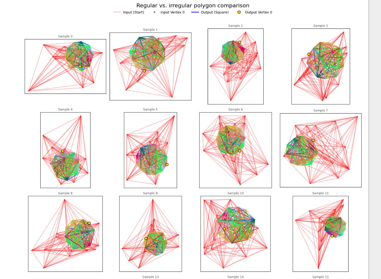
So how does the model do? Well, here’s a visualization of a random quadrilateral being passed through my SquareModel:

Just Look at that big, beautiful square!

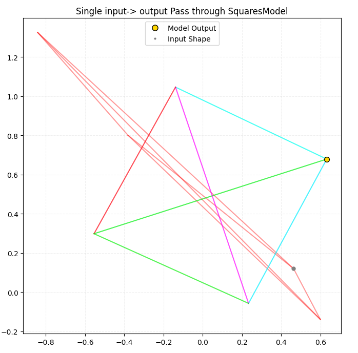
Damn, that was satisfying. Alright, let’s do it 20 more times.

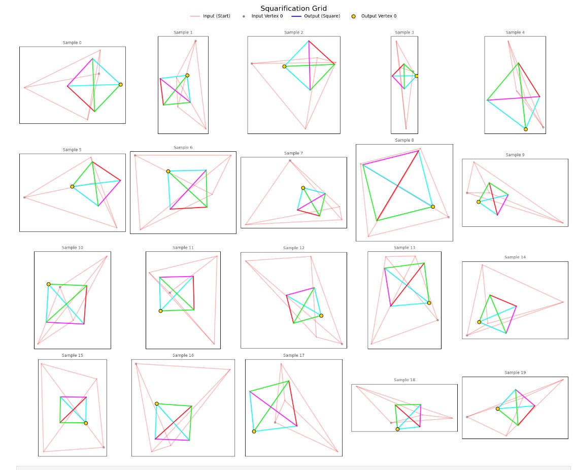
But notice something important about the squares being generated. Specifically, look at the colors of the output square edges. I color-coordinated these edges based on the winding order. Essentially, when we encode our quadrilaterals as an array A, I made sure to color the connection between A[0] and A[1] using the same color for every shape. If my model had learned to transform the points into a square with a given point order (e.g. [bottom-right, upper-right, upper-left, lower-left]), then every generated square would have the same edge colors.

But they don’t! Some squares have a green diagonal, while others have red, blue, or magenta diagonals. This means that my model is able to recognize a square regardless of the order of its elements.

Permutation Equivariance!

And look at the little dots on the corners. Those represent the “starting point” (the bottom left corner) of the input. If my model preferred to orient squares in any particular way, there would be a noticeable pattern in how these corners were arranged. But there’s not!

E(2) Equivariance! This is precisely what I set out to achieve.

Now that I’ve learned how to build a simple EGNN layer, I can start to work on incorporating it into a larger diffusion model, and using that model to generate climbs.

I couldn’t help myself but generalize it to any number of points. Here’s pentagons!

and here’s 16-gons. That’s-a-spicy-meat-a-ball!

If you have any questions for me about this topic, or if you have any ideas for other topics I could explore, leave a comment below!

Stay curious!

1. However, matching nodes must be identical, and that includes whatever additional data is attached to each node. For example, if the goal-keeper and the center striker on a soccer team swap places, then the point cloud describing the team’s position has changed, even if the ‘set of coordinates’ is the same. This is because two coordinates have effectively swapped information (The coordinate formerly containing ‘center striker’ now contains ‘goalkeeper’).

1.

2. Why?

1. If you think of the final distribution as being a PDF, the diffusion model needs to take data located at some random point in space and move it upslope towards points of greater likelihood. In order to do that, it needs to know the direction in which the denser regions lie relative to the starting point. This is not invariance, but equivariance. For example, if the target distribution is permutation invariant, then [p1, p2, p3, p4] and [p4, p2, p1, p3] should be equally likely: that’s invariance. However, the direction in which our model updates the noisy data [p1’->p1, p2’->p2, p3’->p3, p4’->p4] should depend on the points’ order.

f(p1', p2', p3', p4') = [p1, p2, p3, p4]
f(p2', p3', p1', p4') = [p2, p3, p1, p4], not [p1, p2, p3, p4]

Invariant outcomes require equivariant transformations.

3. This idea, and most of my understanding of these models, comes from the paper E(n) Graph Neural Networks (Satorras, Hogeboom, Welling). Their model also formed the basis for my torch EGNN model. You can look through their codebase here.

4. (I hate that Substack doesn’t support inline LaTeX)

5. Note that if we were to include the exact coordinates of either A or B in this message construction, we would lose E(n) Equivariance. Why?

Well, there’s no guarantee that, for example, NN([0,0],[1,1],...) will return the same result as its reflection over the x-axis, NN([0,0],[-1,-1],...). Neural networks have few built-in symmetries. To guarantee E(n) Equivariance, we cannot use spatial features directly. However, we made no such guarantees about non-spatial features, so they’re fair game.