BetaZero V2: A Diffusion Model for setting Boulder Problems
My journey building a custom DDPM for generating realistic board climbs, from scratch.

The next chapter in the Beta-Zero saga!
When I last wrote about this project, I was using an auto-regressive LSTM model to generate realistic board climbs on my home wall. After about 40 hours of testing, training and tweaking, I was able to set reasonable looking “climbs” as sequences of moves.
Problems with the LSTM Approach
However, the LSTM climb-generator proved weak on several fronts.
Memory: Despite the name, my “Long-short-term memory” model seriously struggled to recall which holds had previously been part of the sequence. It had a tendency to “meander” around the board and recycle holds it had already used.
Variety: The LSTM is trained to find the “correct” next position from a given input position. This tends to result in the same hold sequences appearing 100% of the time for a given set of starting holds. I could mitigate this behaviour by increasing the model’s “temperature” (adding random noise to its outputs), but this significantly lowered the quality of the generated climbs.
Finally, my training dataset was awful: It contained just 30 real climbs, along with 40 more “couch-sets” which I had never tested IRL but assumed were doable.
However, right as I was finishing up my LSTM model, I stumbled upon an open-source API which would change everything.
Boardlib.
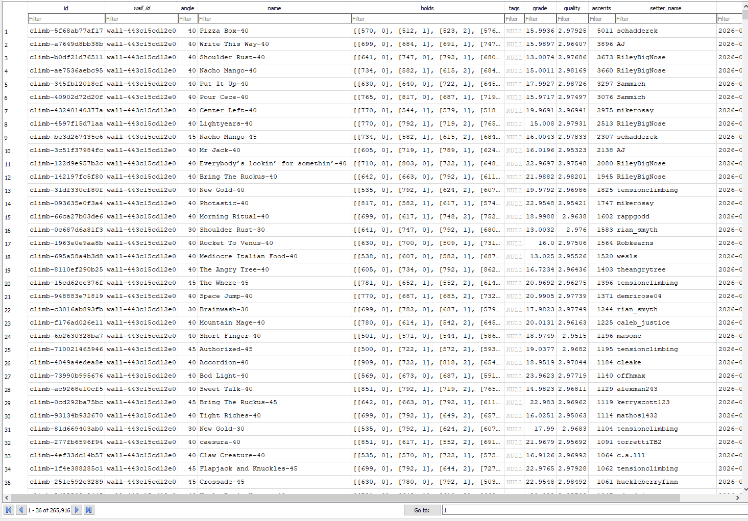
Boardlib is an open-source Python API for accessing and analyzing public board climbs and ascents.
Boardlib provides access to public climbs from Kilter, Tension, Decoy, Moonboard, and even some really niche system boards (What the hell happened to GrassHopper?).
But there was one big problem with this dataset: Boardlib climbs have no inherent sequence — they’re simply stored as an assortment of holds and roles (Hand, Foot, Start, Finish). How can I train a sequential model to generate a sequence of holds if I don’t know what sequence the holds are supposed to go in?
Enter: Denoising Diffusion Probabilistic Model (DDPM)

Yep, it’s time to explain diffusion. A Denoising Diffusion Probabilistic Model (DDPM) is a specific architecture of generative AI which attempts to mimic, and then reverse, the physical process of diffusion.
Diffusion iteratively adds noise to a clean dataset, gradually “diffusing” it throughout feature-space. The core conceit of DDPMs is that training a model to incrementally “denoise” data will eventually allow it to reconstruct the original data distribution from an input of pure static.
The architecture of a DDPM
Forward diffusion
The first thing our DDPM needs is a forward diffusion process, which is some function that adds a set amount of gaussian noise to the original dataset. Here’s the naive implementation of a gaussian noise function:
However, in practice, it’s quite cumbersome to call the same function repeatedly, adding just a little bit of Gaussian noise each time. Instead, we can take advantage of the fact that Gaussian noise is additive: The sum of identical gaussians is simply a bigger gaussian1. Therefore, rather than summing t small gaussians, we just scale our noise by t.
Noise schedule
In practice, it’s often useful to maintain variance as we diffuse our dataset. Therefore, rather than simply Gaussian noise to the original distribution, we can gradually substitute the raw data for Gaussian noise.
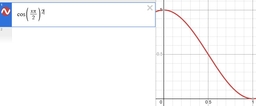
Where a is a function of t which maps to the range [0,1]. While alpha can simply be equal to t, in practice people usually choose a scheduling function with smoother gradients close to t=0 and t=1. For example, a cosine schedule gives the model more timesteps to work on “finishing touches”, and it’s what I used in ClimbDDPM.
Denoising model
The denoising model attempts to predict the noise added during each timestep of the diffusion process.
Why predict the noise?
Now, this might seem pedantic, but trust me, it’s important. The denoising model in a DDPM should predict the normalized Gaussian noise added at each timestep, not the ‘clean data’. “But isn’t that the same thing?”, I hear you protest.
No. The difference becomes apparent when we approach t=0. Because we scale our noise with t, at low t values, the loss associated with changes in our noise N approaches 0, and model learns to just predict “no noise”.
But for our noise prediction model, t=0 is actually the hardest timestep to predict. Even though only a small amount of noise was added, the loss associated with that noise is the same magnitude as it is for every other timestep.
By training our model to predict the normalized gaussian noise, we essentially grant equal importance to each diffusion step. This means our model won’t “slack off” as the generated dataset approaches our true distribution; rather, it will diligently fill in the details as accurately as it can.
ClimbDDPM: Building a custom DDPM in python.
Denoising Model: Convolutional U-Net
There are many possible architectures for the denoising model: U-Net, EGNN (see “Can an AI Generate Squares”), Transformer, Set Transformer, etc. I spent probably 20-30 hours testing out various different architectures. I eventually settled on a convolutional U-Net design, because it was the most easy to implement and consistent to train.

The U-Net architecture is designed to capture both general and individual properties of an ordered input sequence S, of length N and hidden dimension D2. The “U” in U-net refers to the compression and decompression that happens between the first and last layers. The first half of the layers in the U-Net compress information down into a dense, compact “latent” space L, with a much smaller length and a much greater hidden dimension.
The latent space “squeezes” the sequence, and forces the model to learn general properties rather than memorizing. However, we don’t want to “destroy” the finer details of the dataset when we compress it into the latent space. Therefore, we retain Skip Connections connecting each successive “down block” to the corresponding “up block” of the same size. This allows our U-Net to capture both general information and finer sequence detail. While most U-Nets use input concatenation in their skip connections, I used input summation, essentially transforming my skip connections into a residuals architecture. I personally found this architecture to be more friendly during model training, and it also lowered the parameter-size of my denoising model considerably. However, I would like to test the efficacy of residuals vs. input concatenation in my next iteration of ClimbDDPM.
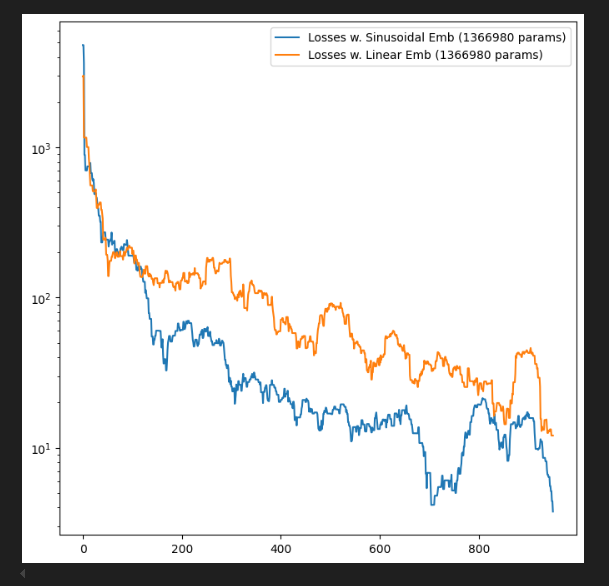
Embedding Strategy: Sinusoidal t, Cond. MLP
I also tested various ways of embedding the hold-set (x), conditional features (c), and time-step (t) in my model. I eventually settled on a Sinusoidal Time Embedding3, and a linear MLP for embedding conditional features c.
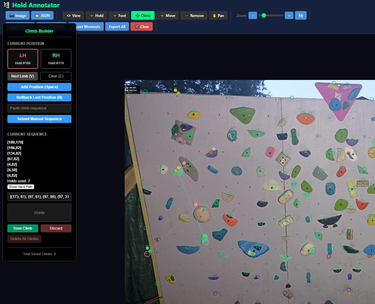
I embedded climbing hold-sets as Sequences of dimension [20,4], excluding all climbs of length > 20, and padding all shorted climbs with null holds. This allowed me to train my model on batched climb data, of shape [B, 20, 4], along with c of shape [B, 4] and t of shape [B, 1].
Generating Climbs with the DDPM
To generate a climb with our DDPM, we start with a vector consisting of random gaussian noise, and set t to 1. Then we ask our denoising model “What noise did we add to a real climb at time t to get this noisy climb?”. We can then use this estimate of N to recover an approximation of the original climb.
Then we decrement the time t, and re-noise our estimate, but by slightly less this time.
Note that we can re-use the original noise N, or generate new Gaussian noise to add, during this step. I prefer adding new noise because it increases the Variety of generated climbs, while maintaining our model’s expected performance.
After 100 timesteps, our diffusion model will have taken a set of random coordinates and transformed them into a “valid” set of climbing holds!
The final piece: Projected Diffusion
However, there is one flaw which makes vanilla DDPM incompatible with generating board climbs. Diffusion operates on a continuous space, while board climb hold-sets are fundamentally discrete. To solve this issue, I implemented projection.
The idea of projection is super simple. At each step in the diffusion process, project each generated hold onto the real hold which is “closest” to it. The main fear with this strategy lies in how we define “close”. While a real hold may be physically close to the model’s generated hold, pulling it onto the real hold may significantly degrade the “validity” of the generated climb (e.g. the DDPM wants to place a Jug at one position, but the projection step projects it onto a foot-hold.). Additionally, if we wait until the very end of the DDPM Generation process to perform projection, there may be no configurations of real holds which are close to the climb generated by the DDPM.
There are more sophisticated solutions to these problems, but for now I attempted to solve them by using a projection schedule similar to the denoising schedule shown above. Each guess is interpolated between a projection onto the real holds RH, and our original guess x_t.
As t approaches 0, we weight the projection more heavily until, during the final generation step, we just return project(x, RH).
Visualizing the Diffusion Process
By setting the re-noising process to deterministic and tracking the ‘renoised’ climbs at each step, we can actually see the climb “building itself” during the reverse diffusion process! See how the holds are either pulled off-screen (to “null-sentinels” [-2,0] and [2,0]), or join together to build the final climb!
Here we can see what happens when we add projection. You can see that the “sudden” onset of the projection seriously messes with the reverse diffusion process. It seems, however, that a good solution is to add mild projection early on in reverse diffusion:
I’m still working out the optimal projection schedule for ClimbDDPM. I’m also working on adding better Conditional Generation. Finally, I want to include hold classification as a conditional input in the DDPM. In fact, it baffles me that I didn’t think to include it as conditional input in the first place (I got kind of obsessed with Discrete Absorbing Diffusion, which ended up being largely unnecessary for this type of problem).
The exact formula states that adding n identical Gaussian distributions will result in a new Gaussian with n times the mean and variance:
If you’re wondering what I mean by “hidden dimension”: I mean how many unique pieces of information (features) are stored in each “element” of the sequence. So for an RGB picture, the “hidden dimension” is initially 3: the R, G, and B values of each pixel. Neural networks usually expand this hidden dimension, e.g. each “pixel” is represented by 128 unique values rather than just 3. This allows the network to encode more complicated properties of the data. People also use the term “Feature Dimension” when referring to datasets, but “Hidden Dimension” is more popular when referring to model architecture.
Sinusoidal Embedding is an algorithm for converting a simple linear distribution into a cyclic distribution with many different cyclic “periods”. Essentially, this embedding allows our “time” input to capture changes occurring on multiple different timescales. This is useful because sometimes we want our model’s behavior to change drastically depending on the timestep. If our time input was just a simple linear embedding, the embedding for t=0.1 and t=0.08 would only differ by a tiny amount, and our model would struggle to “learn” to treat these two timesteps differently. This article brilliantly explains the utility of Sinusoidal Embeddings and the reasoning behind them.